Subgroups.Rmd

---
title: "Práctica de Descubrimiento de Subgrupos"
author: "Javier Galván Fraile - Jorge Medina Hernández"
date: "4/19/2020"
output: 
  html_document:
    toc: true
    number_sections: true
---

```{r setup, include=FALSE}
knitr::opts_chunk$set(echo = TRUE)
```

# Exercise 1.

Los Angeles es la ciudad más grande del estado de California y es el hogar de aproximadamente 17 millones de personas. Es famosa por ser el centro de la producción de cine y televisión estadounidenses en Hollywood, así como el hogar de muchas celebridades. La mayoría de las actividades turísticas están conectadas a la industria cinematográfica (Universal Studios, Disneyland en el cercano Anaheim, Hollywood Walk of Fame ...), aunque la ciudad tiene algunas playas hermosas en el Pacífico. En cuanto a la seguridad, Los Angeles no tiene punto medio: mientras que la mayoría de los barrios turísticos como Hollywood, Beverly Hills o Santa Mónica son seguros, tiene algunas áreas muy peligrosas en el centro (Skid Row) y cercanas (South Central).

En esta práctica, usaremos la base de datos de crímenes desde el 2010 hasta la actualidad proporcionada por el Departamento de Policia de Los Angeles. Esta base contiene las características de cada delito ocurrido en la ciudad de Los Angeles desde 2010. Estos datos se han transcrito a partir de los informes elaborados por la policia en papel por cada delito. Se puede descargar desde el enlace: https://data.lacity.org/A-Safe-City/Crime-Data-from-2010-to-Present/y8tr-7khq. Recoge alrededor de
1.9 millones de incidentes criminales con 26 variables de distintos tipos. Sin embargo, usaremos solamente los datos correspondientes al año 2019.

A partir de esta base, el objetivo principal es:

* Descubrir subgrupos en los datos que puedan resultar de interés y su posterior interpretación

Se valorarán los siguientes aspectos:

  1. Calidad de los subgrupos encontrados, su interés e interpretación.
  2. Uso de diferentes algoritmos de descubrimiento de subgrupos.
  3. Uso de distintas medidas de calidad.
  4. Implementación de alguna medida de calidad distinta de las consideradas en el paquete rsubgroup y aplicación de la misma a las reglas obtenidas en base a otras medidas sí contempladas en el rsubgroup.

La práctica se realizará en grupos de 2-3 estudiantes y se deberá entregar un Rmd que incluya las instrucciones usadas, así como la memoria de la práctica. Se valorará especialmente el análisis de los resultados obtenidos.

## Dataset analysis

### Feature selection

In this task we will use the [crime database]( https://data.lacity.org/A-Safe-City/Crime-Data-from-2010-to-2019/63jg-8b9z) from the Police Department of Los Angeles, which describes the features of each crime committed in LA between 2010 and 2019, although we will only analyze the ones which took place along 2019. The main goal is to discover subgroups among data and analyze their quality, interest and interpretation. 

Firstly we will directly load the data from 2019 alone and show its first rows as an example to see how it is structured.

```{r}
DB <- read.csv(file='Crime_Data_2019.csv')
head(DB)
```

Let's get some insight about the different crimes by looking at the statistical properties of the different attributes 

```{r}
summary(DB)
```

We observe that we have such a large number of features that we must select the most appropiate ones for our study in order to extract useful information from them. Thus, from the different attributes that characterise a crime we are focusing on 1 or 2 per group of features:

  1. **Time features**. We are only going to work with the time ('TIME.OCC') and date ('DATE.OCC') at which the crime took place. The neglected time feature is the time at which it was reported to the local Community Police Station ('Date.Rptd') as we consider that this feature is less useful than the time at which the crime took place.
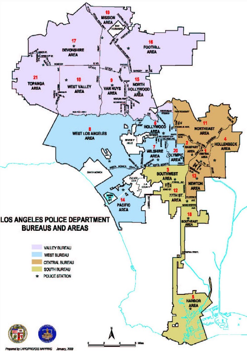
  2. **Spatial features**. From this field we will pay special attention to the geographic area of the local Community Police Station where the crime was commited ('AREA.NAME') which are shown in the following map. Also we will take into consideration the place where the crime occurred ('Premis.Desc'). Other features like 'AREA', which represents the numeric label of the area, are not considered. Also we consider that the reported district number ('Rpt.Dist.No'), which represents the sub-area within the area where the crime occurred, has less importance than the area itself and thus we will not take it into account. For this same reason we will not consider the latitude ('LAT'), the longitude ('LON'), the cross street of rounded address ('Cross.Street') and the street address of the crime incident ('LOCATION').
  
  
  ![Map of the geographic area of the Community Police Stations in the City of Los Ángeles. Retrieved from https://www.qsl.net/n6uru/images/lapdcitymap2009.jpg . ](https://www.qsl.net/n6uru/images/lapdcitymap2009.jpg)
  
  
  3. **Victim details**. From this field we will work with the victim age ('Vict.Age'), the victim sex ('Vict.Sex') and the victim descent ('Vict.Descent') as one of our goals is to identify groups of people that are more susceptible to suffer a crime.
  
  4. **Type of crime**. Among the several features that are provided we will focus on the crime committed ('Crm.Cd') and the weapon used ('Weapon.Desc'). Other features like 'Mocodes' are so specific that will require a lot of work in order to extract useful information to discover subgroups from it. The same happens for the less important crimes commited by a criminal ('Crm.Cd1', 'Crm.Cd2', 'Crm.Cd3' and 'Crm.Cd4').
  
Consequently, in our analysis we will restrict to some crime features that seem to be the more relevant, which are the following

```{r}
good_attributes <- c('Weapon.Desc','Vict.Sex', 'Crm.Cd.Desc', 'Vict.Age', 'Vict.Descent', 'TIME.OCC','DATE.OCC', 'AREA.NAME', 'Premis.Desc')
print(good_attributes)
```

We must point out that a more exhaustive analysis of the crimes should consider those attributes that we have neglected. However, as an educated approach we will focus on the above-mentioned.


### Discretization

There are some attributes which require a discretization of the possible values in order to extract useful information of them. In particular, we will discretize the hour at which the crime took place in intervals of 4 hours. With respect to the date the crime took place we will focus on the month and discretize the dates of the dataset into the 12 months.

```{r}
library(varrank)
library(stringr)
library(arules)
```

```{r}
#DISCRETIZE TIME.OCC
#We must first pad the military time with zeros, for which we need string characters
times <- DB$TIME.OCC
times.str <- unlist(strsplit(toString(times),", "))
times.padded <- str_pad(times.str, width = 4, side="left", pad="0")
#Now the first two digits are the #hours, and we have to add them the contribution from the minutes
time.split <- strsplit(times.padded, "")
h1 <- lapply(time.split,'[', 1)
h2 <- lapply(time.split, '[', 2)
min1 <- lapply(time.split,'[', 3)
min2 <- lapply(time.split,'[', 4)
hours <- as.numeric(paste0(h1,h2))
mins <- as.numeric(paste0(min1,min2))
processed.time <- hours + mins/60
times.discretized.big =discretize(processed.time,method="interval",breaks=6, include.lowest = TRUE, right=TRUE)
#times.discretized <- unlist(discretization(data.df = processed.time, discretization.method = "fd", frequency = FALSE))
DB$TIME.OCC <- times.discretized.big

#DISCRETIZE DATE.OCC
#Finally we will discretized dates by month
dates.str <- times.str <- unlist(strsplit(toString(DB$DATE.OCC),", "))
date.split <- strsplit(dates.str, "")
d1 <- lapply(date.split,'[', 1)
d2 <- lapply(date.split, '[', 2)
months <- as.factor(paste0(d1,d2))
DB$DATE.OCC <- months
```

## Subgroups
```{r eval=FALSE, include=FALSE}
Sys.setenv(JAVA_HOME="C:/Program Files/Java/jdk-13.0.2/")
library(rsubgroup)
```

For the purpose of identifying the subgroups we have defined the function `Subgroups.finder`, which uses `DiscoverSubgroups` from the 'rsubgroup' library for the subgroups mining and records the results in csv files. It contains the following arguments:

<table style="width:100%">
  <tr>
    <td> `data.base` </td>
    <td > A data.frame in which perform the subgroups search.</td>
  </tr>
  <tr>
    <td>  `target.attribute` </td>
    <td>Target attribute to consider for subgroup discovery.</td>
  </tr>
  <tr>
    <td> `target.value` </td>
    <td >  Level within the target attribute to consider for subgroup discovery.</td>
  </tr>
    <tr>
    <td> `antecedent` </td>
    <td >List of attributes to consider for mining.</td>
  </tr>
    <tr>
    <td> `method` </td>
    <td >Mining method; one of Beam-Search `beam`, BSD `bsd`, SD-Map `sdmap`, SD-Map en-
abling internal disjunctions `sdmap-dis`.</td>
  </tr>
   <tr>
    <td> `quality` </td>
    <td > Quality function; one of: Binomial-Test `bin`, Chi-Square-Test `chi2`, Lift `lift`, Piatetsky-Shapiro `ps`, Gain `gain`, Relative Gain `relgain`, Weighted Relative Accuracy `wracc`.</td>
  </tr>
   <tr>
    <td> `path.csv` </td>
    <td > Path for the creation of a csv file containing the subgroups found.</td>
  </tr>
</table>
<style>
.tab {border-collapse:collapse;}
th, td {
  padding: 10px;
}
</style>

<p style="margin-bottom:0.25cm;">  </p>

The function outputs two csv files: one containing the subgroups found and located in the desired path `path.csv`, and a second one in `path_info.csv` including the arguments used for the subgroups search. Lastly, since we were obtaining a large number of rules linked to unlabeled data (for instance the value " " from  'Weapon.Desc'), we decided to filter the data base prior to the search; removing the rows related to unknown values of a given feature provided it was part of the antecedent or the target value, i.e. whenever we were focusing on this specific attribute for the subgroups discovery. The classes affected by this process are 'Weapon.Desc','Vict.Sex', 'Vict.Descent' and 'Vict.Age'. In the case of the latter there was a disproportional amount of crimes against people with 0 years of age, as we will show below.

```{r}
hist(DB$Vict.Age, breaks=100, xlab = "Age of the victim", main="Histogram - Age of the victims" )
```

The most likely explanation is that the police department used "0" as a label for "unknown", specially taking into account the type of crimes committed against them. As an example, we will show the top 5 kind of crimes they suffered:

```{r}
crimes.to.0years <- unlist(table(DB$Crm.Cd.Desc[DB$Vict.Age==0]))
print(crimes.to.0years[order(crimes.to.0years,decreasing = TRUE)][1:5])
```

As we see they can not be related to people of 0 years of age. Lastly, after filtering the age we discretized it in intervals of 10 years of length.
```{r}
library(rsubgroup)
Subgroups.finder <- function(database, target.attribute, target.level , antecedent,method,quality,path.csv){
  DB.MOD <- data.frame(DB)
  #We get rid of bad labeled of unlabeled victim sex
  if (target.attribute=="Vict.Sex" | sum(antecedent=="Vict.Sex")>0) {
  DB.MOD <- DB.MOD[(DB.MOD$Vict.Sex!='X' & DB.MOD$Vict.Sex!='' & DB.MOD$Vict.Sex!='N' & DB.MOD$Vict.Sex!='H'),]
  }
  #We now clean the 0 ages
  if (target.attribute=="Vict.Age" | sum(antecedent=="Vict.Age")>0) {
  DB.MOD <- DB.MOD[DB.MOD$Vict.Age!='0',]  
  #Discretizamos las edades
  DB.MOD$Vict.Age=discretize(DB.MOD$Vict.Age,method="interval",breaks=10,include.lowest = TRUE, right=TRUE)
  }
  if (target.attribute=="Weapon.Desc" | sum(antecedent=="Weapon.Desc")>0) {
  DB.MOD <- DB.MOD[DB.MOD$Weapon.Desc!="",]
  }
  if (target.attribute=="Vict.Descent" | sum(antecedent=="Vict.Descent")>0) {
  DB.MOD <- DB.MOD[DB.MOD$Vict.Descent!="" & DB.MOD$Vict.Descent!="X",]
  }
  
  subgroups.found=DiscoverSubgroups(DB.MOD,as.target(target.attribute,target),
                                  new("SDTaskConfig",attributes=antecedent,method=method,qf=quality))
  write.csv(ToDataFrame(subgroups.found),path.csv)
  #Now we will construct the second data frame containing the information of the subgroups search.
  headings <- c("Target attribute","Target value", "Antecedent","Method","Quality")
  data <- c(target.attribute,target.value,paste(antecedent, collapse=","), method,quality)
  config <- data.frame(headings,data)
  #Now the name of the second file
  infoname<- unlist(strsplit(path.csv,""))
  infoname <- paste0(infoname[-length(infoname)+3:-length(infoname)],collapse="")#delete .csv
  infoname <- paste0(infoname, "_info.csv",collapse="")
  write.csv(config,infoname)
  #Print the result also on the screen
  ToDataFrame(subgroups.found)
  }
```

### Latins

In the first part of this project we will focus in analyzing the level of security of different areas in Los Ángeles and try to relate these results to the presence of street gangs in the city. The County and the City of Los Angeles has been nicknamed the "Gang Capital of America," with an estimated 450 active gangs with a combined membership of more than 45,000 in 2019.  Particularly, near the intersection of 18th Street and Union Avenue in downtown Los Angeles, we have the largest street gang of the city with around 15,000 members known as "18 Street", which is mainly formed by latin people. Other relevant latin street gangs are 204th Street Gang (Mexicans), La Mirada Locos (Hispanic), Avenues (Mexicans), Canoga Park Alabama (Hispanic) and Mara Salva Trucha (Salvadoran, Guatemalan and Honduran). We can check the areas where these street gangs habit in the following map.

![Map of street gangs distribution in the City of Los Ángeles. Retrieved from http://blogs.kcrw.com/dna/wp-content/uploads/2018/03/gang_injun_Citywide_2012_2-page-001.jpg ](http://blogs.kcrw.com/dna/wp-content/uploads/2018/03/gang_injun_Citywide_2012_2-page-001.jpg)

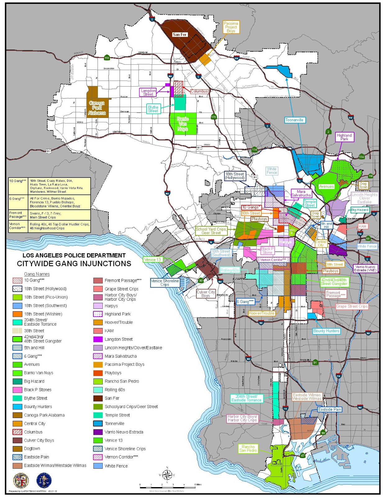
Our objective is now to extract from the dataset potential crimes which involve these latin street gangs and analyze them. For that purpose we will use the function DiscoverSubgroups from the 'rsubgroup' library with the 'sdmap' method and the quality function Chi-Square-Test as well as the Piatetsky-Shapiro quality measurement, given by

$$p s(R)=n(\text { Target}_{\text{value} } \cdot \text { Cond })-\frac{n(\text { Target}_{\text{value}}) \cdot n(\text {Cond})}{n_{s}}$$

where $n_s$ is the total number of examples.

Consequently, we will consider as consequent/target the latin people ('Vict.Descent' = 'H') and as antecedent the following attributes: 'Crm.Cd.Desc', 'AREA.NAME' and 'TIME.OCC'. Thus, we are looking for the worst areas and hours for the latin people as well as the most common crimes they suffer. Notice that we are not considering the weapon used in the crime because in many crimes this data is not proportioned and thus would affect outcoming results by reducing the dataset size.

```{r  eval=FALSE}
latin.1 <- Subgroups.finder(DB, target.attribute = 'Vict.Descent', target.value ='H', antecedent = c('Crm.Cd.Desc', 'AREA.NAME', 'TIME.OCC'), method="sdmap", quality="ps", path.csv = "latin_sdmap_ps.csv")
```

```{r include=FALSE}
latin.1 <- read.csv('latin_sdmap_ps.csv')[-1]
```

```{r}
print(latin.1)
```

We now use as the quality function the Binomial-Test in order to determine how far from random choice are the subgroups found.

```{r  eval=FALSE}
latin.2 <- Subgroups.finder(DB, target.attribute = 'Vict.Descent', target.value='H', antecedent = c('Crm.Cd.Desc', 'AREA.NAME', 'TIME.OCC'), method="sdmap", quality="bin", path.csv = "latin_sdmap_bin.csv")
```

```{r include=FALSE}
latin.2 <- read.csv('latin_sdmap_bin.csv')[-1]
```

```{r}
print(latin.2)
```

Next, we will change the method used to find subgroups by selecting the BSD method and we keep the quality function to be the Binomial-Test.

```{r  eval=FALSE}
latin.3 <- Subgroups.finder(DB, target.attribute = 'Vict.Descent', target.value ='H', antecedent = c('Crm.Cd.Desc', 'AREA.NAME', 'TIME.OCC'), method="bsd", quality="bin", path.csv = "latin_bsd_bin.csv")
```

```{r include=FALSE}
latin.3 <- read.csv('latin_bsd_bin.csv')[-1]
```

```{r}
print(latin.3)
```

Other quality measure functions, like lift or relative gain, give rise to rules with really high accuracy ($\approx 1$) but with a really low support (less than 10 cases overall the dataset). Therefore, the use of these quality measures was really unproductive. Otherwise, with respect to the method used to determine the subgroups, we find that both SD-map and BSD give the same results as expected.

Finally, we are going to consider another quality measurement function. In particular, the quality measurement $Q_c$ which measures the balance between true and false positives as

$$ Q_{c}(R)=T P-c \cdot F P=n(\text { Target}_{\text {value}} \cdot \text { Cond })-c \cdot n(\overline{\text {Target}_{\text {value}}} \cdot \text {Cond}) $$
where $n(\overline{\text {Target}_{\text {value}}} \cdot \text { Cond })=F P$ are the examples satisfying the antecedent but no the consequent and $c$ is a generalization parameter. Particularly, we will take a value $c=2$ in order to penalize those rules that satisfy only the antecedent (false positives).

```{r}
Q.c <- function(p, n.target.cond, c){
  n.cond = n.target.cond/p
  n.notarget.cond <- n.cond-n.target.cond
  q.c <- n.target.cond - c*n.notarget.cond
  return(q.c)
}
```

```{r}
latin.4 <- data.frame(latin.3)
latin.4$quality = Q.c(latin.3$p, latin.3$size, 2)
latin.4 <- latin.4[order(-latin.4$quality),]
print(latin.4)
```

We find that the quality measurement $Q_c$ penalizes rules with a large number of examples but not so high accuracy, pointing out that the most important rule is the one related to crimes suffered in the area of Hollenbeck.

Before analyzing all the rules obtained we must highlight that the percentage of latin people in Los Ángeles is 48.6% (data obtained from the [official census](https://www.census.gov/quickfacts/fact/table/losangelescountycalifornia/RHI725218)), so rules with an accuracy lower than this percentage would not give new knowledge. Then, the most interesting rules obtained are the following:

  1. **Most dangerous zones**. According to all the quality measures we find that the three more important rules by far are those related to areas: 
+ AREA.NAME=Hollenbeck -> Vict.Descent=H; p=0.76, ps=2305.59, bin=28.7
+ AREA.NAME=Newton -> Vict.Descent=H; p=0.66, ps=2396.02, bin=24.99
+ AREA.NAME=Mission -> Vict.Descent=H; p=0.68, ps=2159.93, bin=24.85
  
2. **Most dangerous hours**. We also find that the risk of suffering a crime in the areas above-mentioned increases at certain hours:

+ AREA.NAME=Hollenbeck, TIME.OCC=(20,24] -> Vict.Descent=H; p=0.80, ps=563.05, bin=15.12
+ AREA.NAME=Newton, TIME.OCC=(16,20] -> Vict.Descent=H; p=0.67, ps=567.65, bin=12.48	
+ AREA.NAME=Mission, TIME.OCC=(20,24] -> Vict.Descent=H; p=0.74, ps=545.61, bin=13.67
  
3. **Most common crimes**. Finally, if we focus in the Hollenbeck area, we discover that latin people suffer some characteristic crimes related to assaults:

+ AREA.NAME=Hollenbeck, Crm.Cd.Desc=BATTERY - SIMPLE ASSAULT -> Vict.Descent=H; p=0.84, bin=12.48
+ AREA.NAME=Hollenbeck, Crm.Cd.Desc=INTIMATE PARTNER - SIMPLE ASSAULT -> Vict.Descent=H; p=0.86, bin=10.54
  
From all the rules found we see that the most interesting ones are those related to the area where crimes occurred, presenting high values in all the quality measures. Other more elaborated rules with more than one antecendent show higher accuracy but they are penalized for presenting a smaller sample.

Thus, we conclude that Hollenbeck is a really dangerous region if you are latin. This is not surprising if we take into account that Hollenbeck is a gang-dominated region of Los Angeles with around 31 different gangs (see [*Social network clustering: An analysis of gang networks - K Luh et al.*](https://pdfs.semanticscholar.org/00f8/b898ae247d41b46677a7817418b3d6b2865d.pdf?_ga=2.103997891.2141519570.1586890929-1146159782.1584761722)). Other regions that you should avoid are Newton (neighbour area of Hollenbeck) and Mission, specially in the night. 



### Women

In the second part of this project we will focus in analyzing other of the most vulnerable communities against crime, the female population. In LA around 50.7% of the population are women (data obtained from the [official census](https://www.census.gov/quickfacts/fact/table/losangelescountycalifornia/RHI725218)) and they are susceptible to suffer from gender related violence, specially from their intimate partners. This type of violence covers intimate partner simple asssault under the category of domestic violence including stalking, rape and murder (see  [*As homicides drop in L.A., more women are being killed — often by intimate partners. Los Angeles Times*](https://www.latimes.com/projects/women-violence-homicides-increase-death-murder/)). 

![Poster against gender violence published by Los Ángeles County. Retrieved from http://dpss.lacounty.gov/wps/wcm/connect/1cf5d568-7029-4789-8c0f-7c72b23bb73c/1/dv.jpg?MOD=AJPERES&CACHEID=1cf5d568-7029-4789-8c0f-7c72b23bb73c/1 . ](http://dpss.lacounty.gov/wps/wcm/connect/1cf5d568-7029-4789-8c0f-7c72b23bb73c/1/dv.jpg?MOD=AJPERES&CACHEID=1cf5d568-7029-4789-8c0f-7c72b23bb73c/1)

Our goal is now to discover within the dataset potential crimes suffered by women and analyze them. Consequently, we will consider as consequent/target the female population ('Vict.Sex' = 'F') and as antecedent the following attributes: 'Crm.Cd.Desc', 'Premis.Desc' and 'TIME.OCC'. Thus, we are looking for the most common crimes they suffer as well as the places and hours where they took place. Notice that we are not considering the weapon used in the crime because in many crimes this data is not proportioned and thus would affect outcoming results by reducing the dataset size.

For that purpose we will use the function DiscoverSubgroups from the 'rsubgroup' library with the 'sdmap' method and the quality function Chi-Square-Test as well as the Piatetsky-Shapiro quality measurement.

```{r  eval=FALSE}
women.1 <- Subgroups.finder(DB, target.attribute = 'Vict.Sex', target.value ='F', antecedent = c('Crm.Cd.Desc', 'TIME.OCC', 'Premis.Desc'), method="sdmap", quality="ps", path.csv = "women_sdmap_ps.csv")
```

```{r include=FALSE}
women.1 <- read.csv('women_sdmap_ps.csv')[-1]
```

```{r}
print(women.1)
```

We now use as the quality function the Binomial-Test in order to determine how far from random choice are the subgroups found.

```{r  eval=FALSE}
women.2 <- Subgroups.finder(DB, target.attribute = 'Vict.Sex', target.value='F', antecedent = c('Crm.Cd.Desc', 'TIME.OCC', 'Premis.Desc'), method="sdmap", quality="bin", path.csv = "women_sdmap_bin.csv")
```

```{r include=FALSE}
women.2 <- read.csv('women_sdmap_bin.csv')[-1]
```

```{r}
print(women.2)
```

Next, we will change the method used to find subgroups by selecting the BSD method and we keep the quality function to be the Binomial-Test.

```{r  eval=FALSE}
women.3 <- Subgroups.finder(DB, target.attribute = 'Vict.Sex', target.value ='F', antecedent = c('Crm.Cd.Desc', 'TIME.OCC', 'Premis.Desc'), method="bsd", quality="bin", path.csv = "women_bsd_bin.csv")
```

```{r include=FALSE}
women.3 <- read.csv('women_bsd_bin.csv')[-1]
```

```{r}
print(women.3)
```

Other quality measurement functions, like lift or relative gain, again give rise to rules with really high accuracy ($\approx 1$) but with a really low support (less than 10 cases overall the dataset). Therefore, the use of these quality measures was really unproductive. Notice also that both methods used to determine the subgroups, SD-map and BSD, give the same results as expected.

Finally, we are going to consider again the quality measurement $Q_c$ with a value $c=2$ in order to penalize those rules that satisfy only the antecedent (false positives).

```{r}
women.4 <- data.frame(women.3)
women.4$quality = Q.c(women.3$p, women.3$size, 2)
women.4 <- women.4[order(-women.4$quality),]
print(women.4)
```

The most interesting rules obtained are the following:
  
  1. **Crimes suffered**. According to all the quality measures we find that women are quite more susceptible to suffer certain crimes than men. In particular some important rules according to the Piatetsky-Shapiro quality measure are
  
+ Crm.Cd.Desc=INTIMATE PARTNER - SIMPLE ASSAULT -> Vict.Sex=F; p=0.76, ps=3467.32, bin=31.64
+ Crm.Cd.Desc=VIOLATION OF RESTRAINING ORDER -> Vict.Sex=F; p=0.77, ps=751.17	, bin=14.89
+ Crm.Cd.Desc=INTIMATE PARTNER-AGGRAVATED ASSAULT -> Vict.Sex=F; p=0.77, ps=849.19, bin=15.84	

  Notice that these rules present a high value in the Piatetsky-Shapiro measurement, mainly due to the fact that are laws with a large support. However, if we consider the other three quality measures: the Binomial Test, the Chi-Square-Test and $Q_c$, we find another two important rules with a much lower support but a really large accuracy:
    
+ Crm.Cd.Desc=RAPE, FORCIBLE -> Vict.Sex=F; p=0.99, bin=15.30
+ Crm.Cd.Desc=BATTERY WITH SEXUAL CONTACT -> Vict.Sex=F; p=0.90, bin=14.50	

  These large accuracies highlight the fact that these crimes are suffered almost exclusively by women.
    
2. **Domestic crimes**. Our analysis also shows that most crimes commited in a domestic environment are suffered by women, in particular we find the rules
  
+ Premis.Desc=SINGLE FAMILY DWELLING -> Vict.Sex=F; p=0.57, ps=3882.51, bin=19.78	
+ Premis.Desc=MULTI-UNIT DWELLING (APARTMENT, DUPLEX, ETC) -> Vict.Sex=F; p=0.60, ps=2954.64, bin=19.43	


From all the rules we have found, the most interesting ones are those related to the type of crime suffered by women, presenting high values in all the quality measures. Other more elaborated rules with more than one antecendent present higher accuracy but they are penalized for presenting a smaller sample. The same happens for rules with a smaller sample but with large accuracies. Also, the quality measurement $Q_c$ penalizes those rules with a large number of examples but not so high accuracy, pointing out that the most important rule is the one related to simple assault performed by intimate partners.

We conclude that women are really susceptible to suffer from different type of assaults, including rape and sexual contact, in comparison with men. Furthermore, we observe that these crimes are more prone to happen in a domestic environment.


### Men 

Having analyzed the type of crimes committed against the female population, it is now time to focus on those involving men as victims. According to the [National Gang Center]( https://www.nationalgangcenter.gov/) from the USA, street gangs are conformed predominantly by men. Therefore, the male population would be more prone to take part in violent crimes and murders both as victims and aggressors, [pushing the homicide rate](https://abcnews.go.com/US/story?id=90009&page=1) in the city of LA.

![Distribution of gang members by gender in the USA. Retrieved from https://www.nationalgangcenter.gov/Content/Images/Charts/Demographics-3.png.](https://www.nationalgangcenter.gov/Content/Images/Charts/Demographics-3.png)

Thus, with the intention of verifying the previous statements and discovering other potential type of crimes against men, we will consider as consequent/target the male population (‘Vict.Sex’ = ‘M’) and as antecedent the following attributes: ‘Crm.Cd.Desc’, ‘Premis.Desc’ and ‘TIME.OCC’. Although the weapon used in the crime could be a potential source of knowledge related to gang wars, we have rejected its implication in the analysis due to the lack of information from this specific feature, after veryfing that the rules obtained when considered did not have statistical significance.

As before, we will begin the subgroups discovery using the 'sdmap' method and sorting the results according to the Piatetsky-Shapiro quality measurement.

```{r eval=FALSE} 
men.1 <- Subgroups.finder(DB, target.attribute = "Vict.Sex", target.value= "M",antecedent = c("Vict.Descent","Premis.Desc","Crm.Cd.Desc", "TIME.OCC"), method= "sdmap",quality= "ps", path.csv = "men_sdmap_ps.csv")
```

```{r include=FALSE}
men.1 <- read.csv('men_sdmap_ps.csv')[-1]
```

```{r}
print(men.1)
```

We will now repeat the search using the BSD method keeping Piatetsky-Shapiro as the quality mesurement.

```{r eval=FALSE} 
men.2 <- Subgroups.finder(DB, target.attribute = "Vict.Sex", target.value= "M",antecedent = c("Vict.Descent","Premis.Desc","Crm.Cd.Desc", "TIME.OCC"), method= "sdmap",quality= "ps", path.csv = "men_bsd_ps.csv")
```

```{r include=FALSE}
men.2 <- read.csv('men_bsd_ps.csv')[-1]
```

```{r}
print(men.2)
```

Then, we will change the quality function to Binomial-Test using the BSD method.

```{r eval=FALSE} 
men.3 <- Subgroups.finder(DB, target.attribute = "Vict.Sex", target.value= "M",antecedent = c("Vict.Descent","Premis.Desc","Crm.Cd.Desc", "TIME.OCC"), method= "sdmap",quality= "ps", path.csv = "men_bsd_bin.csv")
```

```{r include=FALSE}
men.3 <- read.csv('men_bsd_bin.csv')[-1]
```

```{r}
print(men.3)
```

As in the previous cases, we notice that both SD-Map and BSD give similar results. Furthermore, since other quality measurement functions implemented in  `DiscoverSubgroups` lead to rules with high accuracy and low support, we will introduce $Q_{g}$, a quality evaluation metric that takes into account the balance between the perfectly classifed examples and the rarity of its distribution. It is given by

$$Q_{g}(R)=\frac{TP}{FP+g} = \frac{n(\mathrm{Target}_{\mathrm{value}} \cdot \mathrm{Cond})}{n(\overline{\mathrm{Target}_{\mathrm{value}}} \cdot \mathrm{Cond}) +g},$$

where $g\in[0.5,100]$ is a generalization parameter. We see that $Q_{g}$ will depend only on $TP/TF= f(p,\mathrm{size})$ if
$$g \ll FP = \Big(\frac{1}{p}-1\Big) \mathrm{size}. $$
As we are interested in rules with high accuracy, we will set as a goal $p^{*}\equiv 0.75$ or equivalently $FP^{*} \simeq 0.3 \mathrm{size}$, and estimating $\mathrm{size}^{*}\equiv 1000$ to be a statistically significant size, we obtain  $FP^{*}\simeq 300$. Therefore, although it is not in the recommended interval, we have chosen $g=300 \simeq FP^{*}$; which allows us to penalyze only the rules with size smaller or of the order of $\mathrm{size}^{*}$, leading to rules with both high accuracy and support.

```{r}
Q.g <- function(p, n.target.cond, g){
  n.cond = n.target.cond/p
  n.notarget.cond <- n.cond-n.target.cond
  q.g <- n.target.cond/(n.notarget.cond+g)
  return(q.g)
}
```

```{r}
men.4 <- data.frame(men.3)
men.4$quality = Q.g(men.3$p, men.3$size, 300 )
men.4 <- men.4[order(-men.4$quality),]
print(men.4)
```

We would like to highlight the following rules:

1. **Crime against minoritary ethnics**. The class "O" from "Vict.Descent" indicates that the victim had a descent different than asian, black, or hispanic among others; a group which constitutes about 9% of the total number of victims. 

<ul style="list-style-type:disc;"> <li>Vict.Descent =O -> Vict.Sex = M; p=0.65, ps=2469.15, chi2=1414.12, bin=17.73, Qg=1.80.</li> </ul>

<ul style="list-style-type:none;"> <li> Thus, we see that if the victim belongs to any of these minoritary groups there is a higher chance that the crime was committed to a man. The rule shows reasonably large quality values, specially in the Piatetsky-Shapiro due to the large support. </li></ul>

2. **Aggravated assaults/deadly weapons**. According to the rules found, these crimes affect predominantly to men. 

<ul style="list-style-type:disc;"> <li>Crm.Cd.Desc=ASSAULT WITH DEADLY WEAPON, AGGRAVATED ASSAULT -> Vict.Sex = M; p=0.73, ps=2131.40, chi2= 1838.72, bin=20.77, Qg=2.51.</li></ul>

<ul style="list-style-type:none;"> <li>There could be many factors contributing to the apppearance of this rule, such as the mentioned street gangs, mainly conformed by men. </li></ul>

3. **Shoplifting**. We have found that men are much more likely to be victims of shoplifting of low valuable material ($950 or below).

<ul style="list-style-type:disc;"> <li>Crm.Cd.Desc=SHOPLIFTING - PETTY THEFT ($950 & UNDER) -> Vict.Sex=M; p=0.83, ps=825.25, chi2=1032.35, bin=15.92, Qg=3.16.</li></ul>

<ul style="list-style-type:none;"> <li> Although the rule has low support in comparisson, the high accuracy and performance in the binomial test and $Q_g$ indicate its relevance. The result is surprising and hard to understand, as in principle it does not seem statistically easier to steal material from men. Possible explanations are that shoplifters might be more compassionate towards women, or male owners could sell material more prone to robbery; but from the data available is not possible to perform a rigorous analysis. </li></ul>


### Time interval (8,12]
We have analyzed the incidence of criminality on every time interval, choosing each of them as the target attribute and taking as antecedent the attributes 'Vict.Sex', 'Premis.Desc', 'Vict.Descent', 'Crm.Cd.Desc'; obtaining interesting results between 8am and 12am.

We will start by exploring the subgroups using the SD-Map algorithm, sorting the results by their value on the Piatetsky-Shapiro quality measurement.

```{r eval=FALSE} 
time.1 <- Subgroups.finder(DB, target.attribute =  "TIME.OCC",target.level = "(8.01,12]",antecedent =  c("Vict.Sex","Premis.Desc","Vict.Descent","Crm.Cd.Desc"),method= "sdmap",quality = "ps",path.csv = "8am_sdmap_ps.csv")
```

```{r include=FALSE}
time.1 <- read.csv('8am_sdmap_ps.csv')[-1]
```

```{r}
print(time.1)
```

Then, using the BSD method keeping Piatetsky-Shapiro as the quality mesurement we obtain the following:

```{r eval=FALSE} 
time.2 <- Subgroups.finder(DB, target.attribute = "TIME.OCC", target.value= "(8.01,12]",antecedent = c("Vict.Sex","Premis.Desc","Vict.Descent","Crm.Cd.Desc"), method= "bsd",quality= "ps", path.csv = "8am_bsd_ps.csv")
```

```{r include=FALSE}
time.2 <- read.csv('8am_bsd_ps.csv')[-1]
```

```{r}
print(time.2)
```

Thus, as in the previous cases the BSD and SD-Map algorithm lead to the same rules. Changing the quality function to Binomial-Test and using the BSD method we get:

```{r eval=FALSE} 
time.3 <- Subgroups.finder(DB, target.attribute =  "TIME.OCC",target.level = "(8.01,12]",antecedent =  c("Vict.Sex","Premis.Desc","Vict.Descent","Crm.Cd.Desc"),method= "bsd",quality = "bin",path.csv = "8am_bsd_bin.csv")
```

```{r include=FALSE}
time.3 <- read.csv('8am_bsd_bin.csv')[-1]
```

```{r}
print(time.3)
```

Lastly, we will evaluate $Q_{g}$ for the set of rules obtained using Piatetsky-Shapiro as the quality metric:

```{r}
time.4 <- data.frame(time.3)
time.4$quality = Q.g(time.3$p, time.3$size, 300 )
time.4 <- time.4[order(-time.4$quality),]
print(time.4)
```

As it can be seen, the mayority of the rules concern the **theft of identity**. As stated by the [police department](http://www.lapdonline.org/search_results/content_basic_view/1364) from Los Angeles, the victim of identity theft is a person whose identity has been fraudulently assumed by another with the intent to obtain credit, goods, or services without the victim’s consent. No financial loss is necessary, but is usually linked to this type of crime. It includes the criminal assumption of someone’s name, address, credit card information, driver’s license, social security number and other personal data. Focusing now on two specific rules:

<ul style="list-style-type:disc;"> <li> Crm.Cd.Desc=THEFT OF IDENTITY -> TIME.OCC = (8.01,12]; p=0.43, ps=1939.24, chi2=3092.98, bin=21.37, Qg=0.734.</li> 
<li> Premis.Desc=SINGLE FAMILY DWELLING, Crm.Cd.Desc=THEFT OF IDENTITY -> TIME.OCC = (8.01,12]; p=0.45, ps=1373.81, chi2=2341.02, bin=18.75, Qg=0.782.</li>
</ul>

We see that between 8am and 12am almost half of the identity theft crimes take place, with a significant value for the Piatetsky-Shapiro metric despite the low accuracy; and the greatests $\chi^{2}$ values we have found. Having data from the working hours could be interesting, as based on the crime location and time, it is possible that criminals rely on this information to commit the felonies. Since the police department from LA does not distinguish identity theft cybercrime from the rest, it is also probable that a large proportion of these crimes which took place in family dwellings are of such kind; specially if we take into account that California is the most affected state among the USA in terms of cybercrime:

<tbody><tr>
<td class="tablewrapper">
<table class="tablesorter" style="border-collapse:collapse; width:228pt; border:medium none" width="303">
<thead>
<tr style="height:12.75pt" height="17">
<th style="white-space: nowrap; text-align: center;" class="header">Rank</th>
<th style="white-space: nowrap; text-align: center;" class="header">State</th>
<th style="white-space: nowrap; text-align: center;" class="header">Number</th>
</tr>
</thead>
<tbody>
<tr class=" odd" style="height:12.75pt" height="17">
<td>1</td>
<td>California</td>
<td style="text-align: right;">50,132</td>
</tr>
<tr class=" even" style="height:12.75pt" height="17">
<td>2</td>
<td>Florida</td>
<td style="text-align: right;">27,178</td>
</tr>
<tr class=" odd" style="height:12.75pt" height="17">
<td>3</td>
<td>Texas</td>
<td style="text-align: right;">27,178</td>
</tr>
<tr class=" even" style="height:12.75pt" height="17">
<td>4</td>
<td>New York</td>
<td style="text-align: right;">21,371</td>
</tr>
<tr class=" odd" style="height:12.75pt" height="17">
<td>5</td>
<td>Washington</td>
<td style="text-align: right;">13,095</td>
</tr>
<tr class=" even" style="height:12.75pt" height="17">
<td>6</td>
<td>Maryland</td>
<td style="text-align: right;">11,709</td>
</tr>
<tr class=" odd" style="height:12.75pt" height="17">
<td>7</td>
<td>Virginia</td>
<td style="text-align: right;">11,674</td>
</tr>
<tr class=" even" style="height:12.75pt" height="17">
<td>8</td>
<td>Pennsylvania</td>
<td style="text-align: right;">10,914</td>
</tr>
<tr class=" odd" style="height:12.75pt" height="17">
<td>9</td>
<td>Illinois</td>
<td style="text-align: right;">10,337</td>
</tr>
<tr class=" even" style="height:12.75pt" height="17">
<td>10</td>
<td>Indiana</td>
<td style="text-align: right;">9,746</td>
</tr>
</tbody>
</table>
</td>
</tr>
</tbody>
<div class="tablewrapper-captions">
<p> <small> Based on the total number of complaints submitted to the Internet Crime Complaint Center via its website from each state where the complainant provided state information. Retrieved from [https://www.iii.org/fact-statistic/facts-statistics-identity-theft-and-cybercrime](https://www.iii.org/fact-statistic/facts-statistics-identity-theft-and-cybercrime) </small> </p>
</div>

## Conclusion
We have analyzed the dataset focusing on latin people, gender and the time of occurrence of the crimes. Regarding the first group, we have found a higher criminality towards this community in Hollenbeck, a gang-dominated region. Then, not surprisingly we have confirmed the larger incidence of assaults, rapes and sexual contact suffered by women, being them more prone to happen in a domestic environment; while for men we have seen a greater occurrence of aggravated assaults or assaults with deadly weapons and unexpectedly a higher chance of being shoplifted, as well as a higher general incidence of criminality when the victim belongs to a minoritary ethnic. Finally, we have found a relation between identity theft and the time interval between 8am and 12am.

As possible refinements, we believe that different discretizations could have led to interesting results, such as splitting the dates in seasons or the time of occurrence in morning-noon, afternoon and night. Furthermore, having data from the criminals would have produced higher quality outcomes from a statistical point of view, although this could give rise to discrimination or hate towards people for belonging to a particular social group, for instance the latin community.