DiffGBM

Probabilistic prediction on tabular data with gradient-boosted diffusion and flow-matching models.

DiffGBM estimates the full conditional distribution p(y|x) — not just a point prediction or a Gaussian interval. The distributions it learns can be multimodal, heteroscedastic, skewed, or heavy-tailed, because nothing in the model assumes a parametric predictive family. Training reduces to ordinary LightGBM regression, so there is no neural density estimator to tune.

The API follows scikit-learn conventions and works with sensible defaults.

Installation

pip install diffgbm

Development version:

pip install git+https://github.com/silaskoemen/diffgbm.git@main

Quickstart

We generate a heteroscedastic response with two sinusoidal components and heavy tails.

import matplotlib.pyplot as plt
import numpy as np
from diffgbm import DiffGBM, Samples

seed = 0
rng = np.random.default_rng(seed=seed)
n = 5000
x = rng.uniform(0, 2 * np.pi, size=n)
z = rng.integers(0, 2, size=n)
y = z * np.sin(x - np.pi / 2) + (1 - z) * np.cos(x) + rng.laplace(scale=x / 30, size=n)

Fit the model and draw samples:

model = DiffGBM(seed=seed)
model.fit(x, y)

y_samples = model.sample(x, n_samples=1, seed=seed, verbose=True)
plt.scatter(x, y, s=1, label="observed data")
plt.scatter(x, y_samples[0, :], s=1, alpha=0.7, label="DiffGBM samples")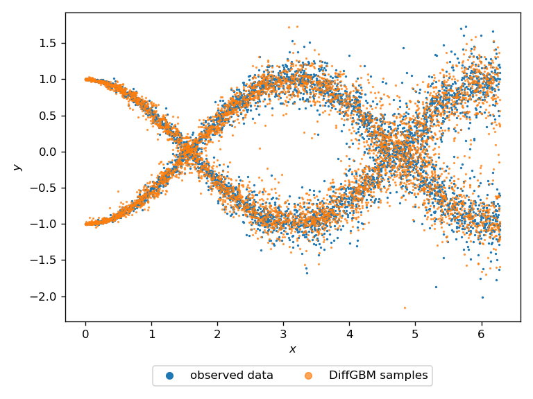

The samples recover both modes and the growing noise scale. Any downstream quantity is then a Monte Carlo estimate:

y_samples = model.sample(x, n_samples=100, verbose=True)  # leading axis is the 100 samples

y_mean = y_samples.mean(axis=0)
y_std = y_samples.std(axis=0)

The Samples helper wraps the common estimators:

samples = Samples(y_samples)
samples.sample_mean()
samples.sample_std()
samples.sample_quantile(q=[0.05, 0.95])

Two operating points

DiffGBM exposes the diffusion path, parameterization, training distribution, features, and sampler as tunable choices rather than fixed defaults. Two configurations are worth knowing about.

Accuracy — score-side recipe (the default). EDM preconditioning, an explicit noise-level feature, log-sigma time sampling, and conditional-mean residualization, sampled with the Euler SDE. In the paper these axes are tuned jointly per dataset ("score-flex"); the defaults are the corner selected on most datasets, so DiffGBM() needs no arguments to get here.

model = DiffGBM(seed=seed)

# the same thing, written out
model = DiffGBM(
    score_parameterization="edm",
    noise_features="raw_time_log_std",
    t_sampling="log_sigma_normal",
    residualize="mean",
    seed=seed,
)

The published Treeffuser recipe is still reachable as an explicit configuration:

model = DiffGBM(
    score_parameterization="noise",
    noise_features="raw_time",
    t_sampling="uniform",
    residualize="off",
    seed=seed,
)

Speed and calibration — flow matching. A directly learned velocity field on a variance-preserving Gaussian path, sampled with a 5-step deterministic Heun ODE. Roughly 5x cheaper sampling than the score path, with the tightest interval coverage.

model = DiffGBM(
    training_objective="flow_matching",
    flow_path="vp",
    seed=seed,
)

Flow matching builds its features from the path itself, so it always uses the raw-time feature layout and ignores the score-only knobs (score_parameterization, noise_features); it warns if you set them.

Categorical features are handled natively — set the column dtype to category in a pandas DataFrame and LightGBM's categorical splits are used directly.

Results

Across eleven tabular benchmarks (nine UCI, including CT-slice localization, and two from scikit-learn), with fold-0 tuning, folds-1–5 evaluation, and an equalized 40-trial budget:

Variant	CRPSS ↑	rel-CRPS ↓	|cE|@90 ↓	sample (s) ↓
Treeffuser (published)	0.699	1.248	0.047	182.7
DiffGBM score-flex	0.725	1.106	0.049	296.1
DiffGBM flow matching	0.707	1.334	0.029	35.5

Score-flex beats the published baseline on every one of the eleven datasets (paired Wilcoxon 11/0, one-sided p = 4.9 × 10⁻⁴), and a DiffGBM row is the per-dataset raw-CRPS winner on 9 of 11.

The two rows are genuinely different operating points rather than one dominating the other. Score-flex buys aggregate accuracy with a stochastic sampler, so it is the slowest row and its interval coverage is no better than the baseline's. Flow matching gives up aggregate CRPS to become the cheapest sampler and the best-calibrated row. Tuned non-diffusion baselines still win individual datasets; see the paper for the full comparison and its caveats.

Documentation

Parameters are documented in the DiffGBM docstring:

from diffgbm import DiffGBM
help(DiffGBM)

Worked examples live in examples/. The research harness that produced the paper's numbers is in benchmarks/, driven by YAML configs under benchmarks/configs/.

FAQ

Sampling is slow. Reduce n_estimators or early_stopping_rounds first. If you need a large speedup, switch to the flow-matching configuration above — it samples in five ODE steps instead of fifty SDE steps.

Citing

If you use DiffGBM, please cite:

@article{koemen2026diffgbm,
  title={Conditioning Tree-Based Diffusions and Flows for Probabilistic Tabular Regression},
  author={Silas Koemen},
  year={2026},
}

DiffGBM builds on Treeffuser, which should be cited alongside it:

@article{beltranvelez2024treeffuser,
  title={Treeffuser: Probabilistic Predictions via Conditional Diffusions with Gradient-Boosted Trees},
  author={Nicolas Beltran-Velez and Alessandro Antonio Grande and Achille Nazaret and Alp Kucukelbir and David Blei},
  year={2024},
  eprint={2406.07658},
  archivePrefix={arXiv},
  primaryClass={cs.LG},
  url={https://arxiv.org/abs/2406.07658},
}

Acknowledgements

DiffGBM is a derivative of Treeffuser by Nicolas Beltran-Velez, Alessandro Antonio Grande, and Achille Nazaret, and retains its gradient-boosted-tree backbone, SDE module, and feature pipeline under the MIT license. See NOTICE for full attribution.

License

MIT — see LICENSE.